


(C) 2013 Lorenzo Peruzzi. This is an open access article distributed under the terms of the Creative Commons Attribution License 3.0 (CC-BY), which permits unrestricted use, distribution, and reproduction in any medium, provided the original author and source are credited.
For reference, use of the paginated PDF or printed version of this article is recommended.
One of the most popular, cheap and widely used approaches in comparative cytogenetics – especially by botanists – is that concerning intrachromosomal and interchromosomal karyotype asymmetry. Currently, there is no clear indication of which method, among the many different ones reported in literature, is the most adequate to infer karyotype asymmetry (especially intrachromosomal), above all in view of the criticisms recently moved to the most recent proposal published. This work addresses a critical review of the methods so far proposed for estimation of karyotype asymmetry, using both artificial and real chromosome datasets. It is shown once again how the concept karyotype of asymmetry is composed by two kinds of estimation: interchromosomal and intrachromosomal asymmetries. For the first one, the use of Coefficient of Variation of Chromosome Length, a powerful statistical parameter, is here confirmed. For the second one, the most appropriate parameter is the new Mean Centromeric Asymmetry, where Centromeric Asymmetry for each chromosome in a complement is easily obtained by calculating the difference of relative lengths of long arm and short arm. The Coefficient of Variation of Centromeric Index, strongly criticized in recent literature, is an additional karyological parameter, not properly connected with karyotype asymmetry. This shows definitively what and how to measure to correctly infer karyotype asymmetry, by proposing to couple two already known parameters in a new way. Hopefully, it will be the basic future reference for all those scientists dealing with cytotaxonomy.
Artificial chromosome datasets, chromosomal heterogeneity, karyotype asymmetry, asymmetry indices, interchromosomal asymmetry, intrachromosomal asymmetry, karyological parameters, Stebbins classification
Cytotaxonomy is a branch of cytogenetics, devoted to the comparative study of karyological features for systematic and evolutionary purposes (
The concept of karyotype asymmetry, i.e. a karyotype marked by the predominance of chromosomes with terminal/subterminal centromeres (intrachromosomal asymmetry) and highly heterogeneous chromosome sizes (interchromosomal asymmetry), was developed for the first time by
Concerning interchromosomal asymmetry, which is due to heterogeneity among chromosome sizes in a complement, other researchers proposed quantitative estimation methods in the following years. This is the case of the Rec index (
More complex and debated is the quantitative estimation of the intrachromosomal asymmetry, which is due to centromere position. To address this issue, the first quantitative index proposed was the TF% of
Finally, a few authors tried to combine the two kinds of asymmetry in a single index, such as
Fundamentally, the basic measures, used in every method proposed so far, are those concerning the length of long (L) and short arm (S) of each chromosome in a complement. All the karyotypes where these measures are not applicable (for instance those with holocentric chromosomes or those with very small chromosomes, 1 µm or less), are not suitable for the estimation of intrachromosomal asymmetry at all. For all the others (the majority), typically L ≥ S ≥ 0 and L ≥ S. The variation extremes are S = L (i.e. chromosomes with centromere perfectly median) and S = 0 (i.e. chromosomes with centromere perfectly terminal). These two variables were combined by researchers in various ways:
L/S also called arm ratio (r), it was used for instance in the widely known chromosome nomenclature proposed by
S/L first proposed by
S/(L+S) also called centromeric index, it is the proportion of short arm respect with the whole chromosome. Its values can range from 0.5 (if S = L) to 0 (if S = 0). It is fundamentally used in TF% = Total length of S in a chromosome set / Total length of a chromosome set × 100 (
L/(L+S) it is the proportion of long arm respect with the whole chromosome, being complementary to the centromeric index. Indeed, [L/(L+S)] + [S/(L+S)] = 1. Its values can range from 0.5 (if S = L) to 1 (if S = 0). It is fundamentally used in AsK% = Total length of L in a chromosome set / Total length of a chromosome set × 100 (
(L–S)/L it was conceived in order to be complementary to S/L, indeed [(L–S)/L]+S/L = 1. Its values can range from 0 (if S = L) to 1 (if S = 0). It is used in A1 = 1 – Mean S/L (
(L–S)/(L+S) it is the difference between the two (complementary) proportions L/(L+S) and S/(L+S). Hence, its values can range from 0 (if S = L) to 1 (if S = 0). It is used in A = Mean (L–S)/(L+S) (
Given that L/(L+S) and S/(L+S) are the only parameters which are formally correct on descriptive statistical grounds (they are both proportions, or relative lengths), and given their peculiar complementary relationships, the only parameter well suited to capture the mean intrachromosomal asymmetry in a karyotype is that proposed by
Comparison of different estimators of intrachromosomal asymmetry on a set of 11 artificial chromosomes with gradually increasing asymmetry, from perfectly median (on the left) to perfectly terminal (on the right) centromeres. Also the mean values are reported in the last column on the right. L/S was excluded because no real value is obtained when S = 0.
| chromosome | ||||||||||||
|---|---|---|---|---|---|---|---|---|---|---|---|---|
| 1 | 2 | 3 | 4 | 5 | 6 | 7 | 8 | 9 | 10 | 11 | mean | |
| S (µm) | 10 | 9 | 8 | 7 | 6 | 5 | 4 | 3 | 2 | 1 | 0 | 5 |
| L (µm) | 10 | 11 | 12 | 13 | 14 | 15 | 16 | 17 | 18 | 19 | 20 | 15 |
| S/L | 1.00 | 0.82 | 0.67 | 0.54 | 0.43 | 0.33 | 0.25 | 0.18 | 0.11 | 0.05 | 0.00 | 0.40 |
| S/(L+S) | 0.50 | 0.45 | 0.40 | 0.35 | 0.30 | 0.25 | 0.20 | 0.15 | 0.10 | 0.05 | 0.00 | 0.25 |
| L/(L+S) | 0.50 | 0.55 | 0.60 | 0.65 | 0.70 | 0.75 | 0.80 | 0.85 | 0.90 | 0.95 | 1.00 | 0.75 |
| (L-S)/L | 0.00 | 0.18 | 0.33 | 0.46 | 0.57 | 0.67 | 0.75 | 0.82 | 0.89 | 0.95 | 1.00 | 0.60 |
| (L-S)/<br/> (L+S) | 0.00 | 0.10 | 0.20 | 0.30 | 0.40 | 0.50 | 0.60 | 0.70 | 0.80 | 0.90 | 1.00 | 0.50 |
Let us return to karyotype asymmetry as a whole, with its two parts: interchromosomal and intrachromosomal. Concerning the measure of interchromosomal asymmetry, as explained above, the main point is to measure how much the chromosome lengths of a complement are different each other, and CVCL (
Concerning the measure of intrachromosomal asymmetry, CVCI should not be used for the reasons explained above. Indeed, it is actually a measure of intrachromosomal heterogeneity, which does not necessarily means asymmetry in the original sense given by
Since the two kinds of asymmetry express different concepts, it is not desirable to combine them in a single value. On the contrary, as argued for the first time by
The present proposal is to couple CVCL with a new parameter called MCA (Mean Centromeric Asymmetry), where Centromeric Asymmetry of a single chromosome is given by the formula (L-S)/(L+S). Accordingly, MCA = A × 100. Generally, CVCI is not correlated with MCA (e.g. in small dataset of Calamagrostis Adanson, 1753 used by
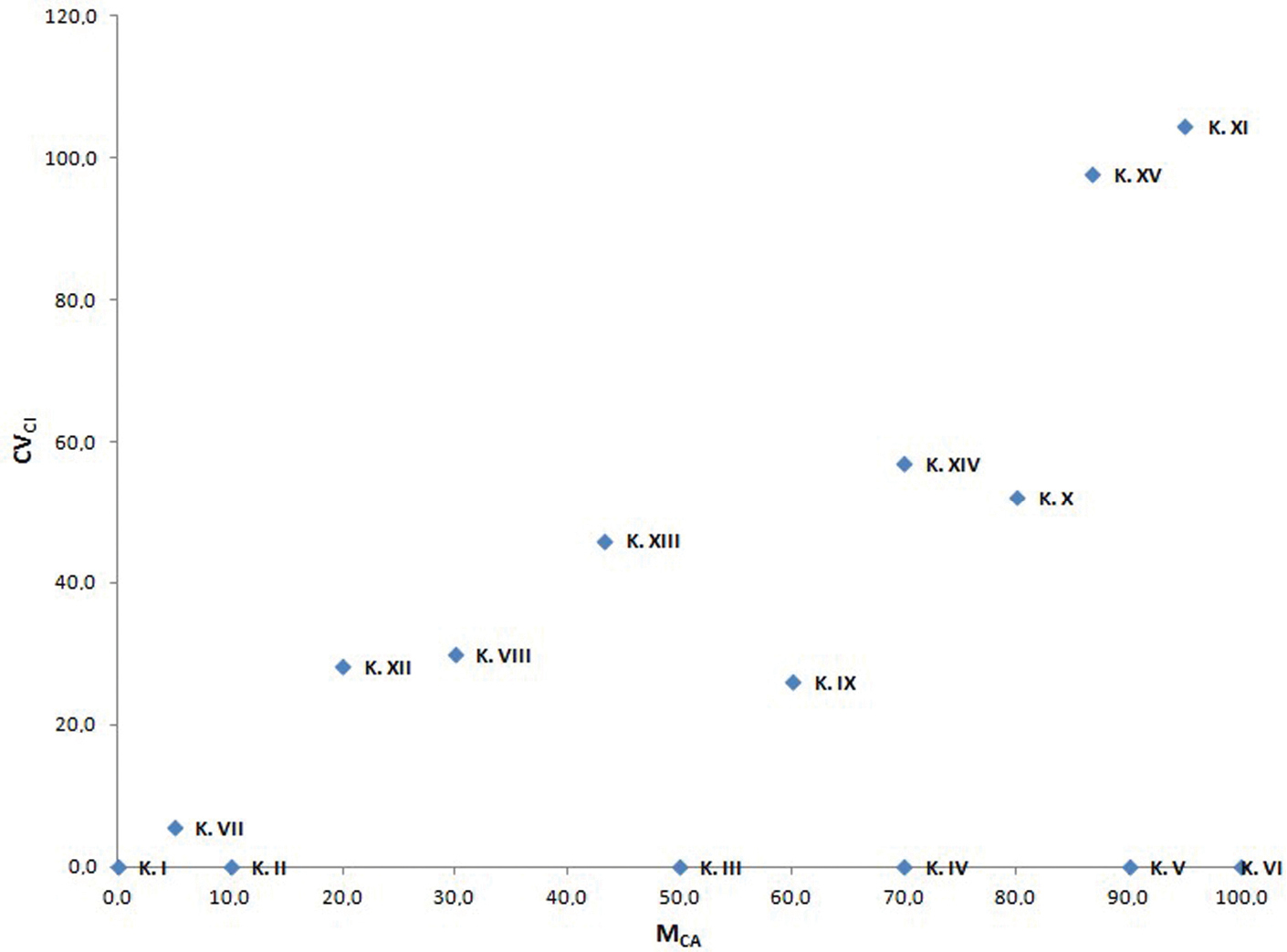
Scatter plot of the fifteen artificial karyotypes reported in Table 2 against MCA (x axis) and CVCI (y axis).
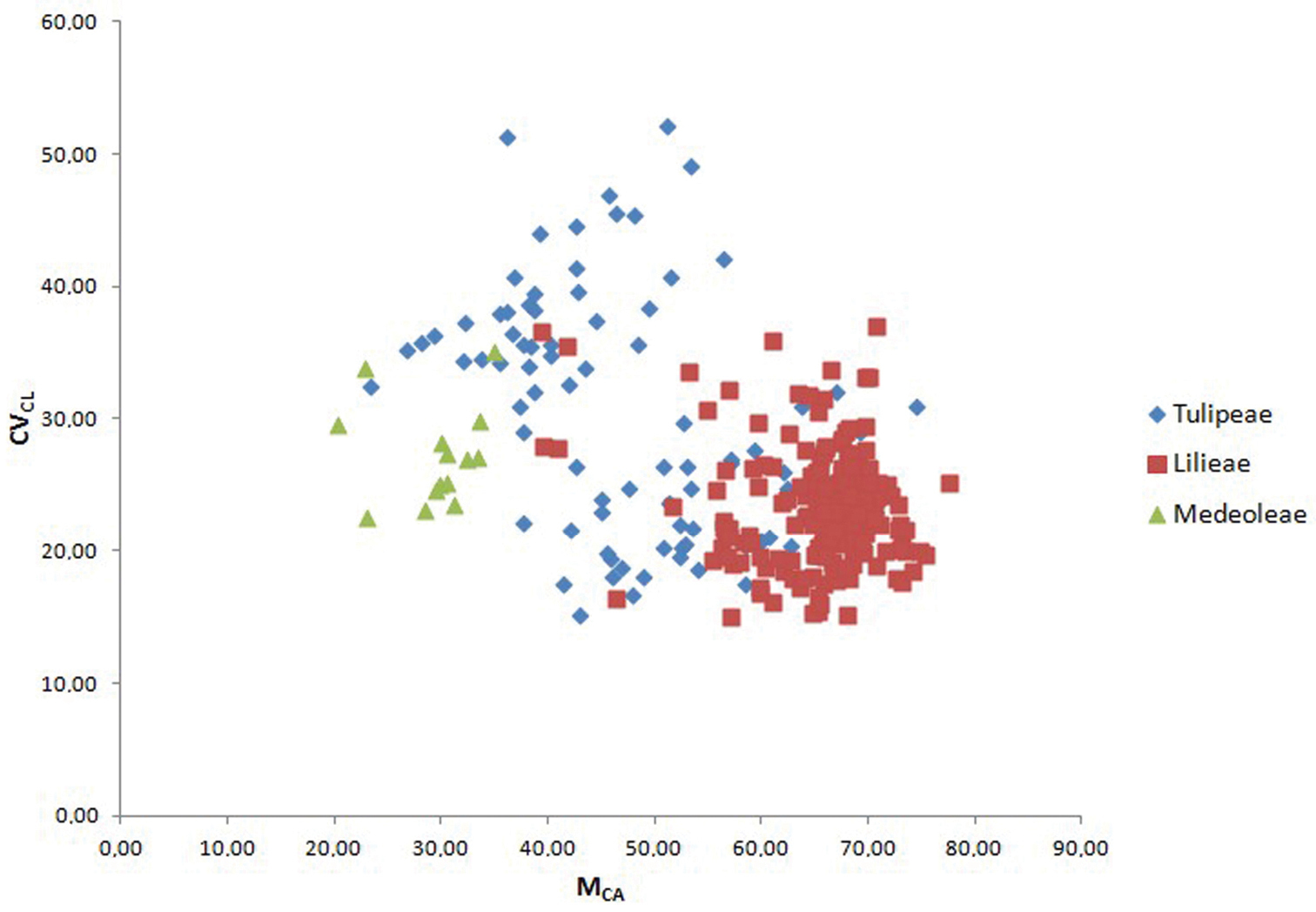
Scatter plot of samples from the three tribes Medeoleae, Tulipeae and Lilieae against MCA (x axis) and CVCL (y axis). Data derived from the dataset published by
Karyomorphometric features of a dataset with fifteen artificial karyotypes, all with the chromosomes of the same length (no chromosome size variation).
| chromosome | ||||||||||||||||||||||||
|---|---|---|---|---|---|---|---|---|---|---|---|---|---|---|---|---|---|---|---|---|---|---|---|---|
| 1 | 2 | 3 | 4 | 5 | 6 | 7 | 8 | 9 | 10 | 11 | 12 | |||||||||||||
| karyotype | L | S | L | S | L | S | L | S | L | S | L | S | L | S | L | S | L | S | L | S | L | S | L | S |
| karyotype I | 5.0 | 5.0 | 5.0 | 5.0 | 5.0 | 5.0 | 5.0 | 5.0 | 5.0 | 5.0 | 5.0 | 5.0 | 5.0 | 5.0 | 5.0 | 5.0 | 5.0 | 5.0 | 5.0 | 5.0 | 5.0 | 5.0 | 5.0 | 5.0 |
| karyotype II | 5.5 | 4.5 | 5.5 | 4.5 | 5.5 | 4.5 | 5.5 | 4.5 | 5.5 | 4.5 | 5.5 | 4.5 | 5.5 | 4.5 | 5.5 | 4.5 | 5.5 | 4.5 | 5.5 | 4.5 | 5.5 | 4.5 | 5.5 | 4.5 |
| karyotype III | 7.5 | 2.5 | 7.5 | 2.5 | 7.5 | 2.5 | 7.5 | 2.5 | 7.5 | 2.5 | 7.5 | 2.5 | 7.5 | 2.5 | 7.5 | 2.5 | 7.5 | 2.5 | 7.5 | 2.5 | 7.5 | 2.5 | 7.5 | 2.5 |
| karyotype IV | 8.5 | 1.5 | 8.5 | 1.5 | 8.5 | 1.5 | 8.5 | 1.5 | 8.5 | 1.5 | 8.5 | 1.5 | 8.5 | 1.5 | 8.5 | 1.5 | 8.5 | 1.5 | 8.5 | 1.5 | 8.5 | 1.5 | 8.5 | 1.5 |
| karyotype V | 9.5 | 0.5 | 9.5 | 0.5 | 9.5 | 0.5 | 9.5 | 0.5 | 9.5 | 0.5 | 9.5 | 0.5 | 9.5 | 0.5 | 9.5 | 0.5 | 9.5 | 0.5 | 9.5 | 0.5 | 9.5 | 0.5 | 9.5 | 0.5 |
| karyotype VI | 10 | 0 | 10 | 0 | 10 | 0 | 10 | 0 | 10 | 0 | 10 | 0 | 10 | 0 | 10 | 0 | 10 | 0 | 10 | 0 | 10 | 0 | 10 | 0 |
| karyotype VII | 5.0 | 5.0 | 5.0 | 5.0 | 5.0 | 5.0 | 5.0 | 5.0 | 5.0 | 5.0 | 5.0 | 5.0 | 5.5 | 4.5 | 5.5 | 4.5 | 5.5 | 4.5 | 5.5 | 4.5 | 5.5 | 4.5 | 5.5 | 4.5 |
| karyotype VIII | 5.5 | 4.5 | 5.5 | 4.5 | 5.5 | 4.5 | 5.5 | 4.5 | 5.5 | 4.5 | 5.5 | 4.5 | 7.5 | 2.5 | 7.5 | 2.5 | 7.5 | 2.5 | 7.5 | 2.5 | 7.5 | 2.5 | 7.5 | 2.5 |
| karyotype IX | 7.5 | 2.5 | 7.5 | 2.5 | 7.5 | 2.5 | 7.5 | 2.5 | 7.5 | 2.5 | 7.5 | 2.5 | 8.5 | 1.5 | 8.5 | 1.5 | 8.5 | 1.5 | 8.5 | 1.5 | 8.5 | 1.5 | 8.5 | 1.5 |
| karyotype X | 8.5 | 1.5 | 8.5 | 1.5 | 8.5 | 1.5 | 8.5 | 1.5 | 8.5 | 1.5 | 8.5 | 1.5 | 9.5 | 0.5 | 9.5 | 0.5 | 9.5 | 0.5 | 9.5 | 0.5 | 9.5 | 0.5 | 9.5 | 0.5 |
| karyotype XI | 9.5 | 0.5 | 9.5 | 0.5 | 9.5 | 0.5 | 9.5 | 0.5 | 9.5 | 0.5 | 9.5 | 0.5 | 10 | 0 | 10 | 0 | 10 | 0 | 10 | 0 | 10 | 0 | 10 | 0 |
| karyotype XII | 5.0 | 5.0 | 5.0 | 5.0 | 5.0 | 5.0 | 5.0 | 5.0 | 5.5 | 4.5 | 5.5 | 4.5 | 5.5 | 4.5 | 5.5 | 4.5 | 7.5 | 2.5 | 7.5 | 2.5 | 7.5 | 2.5 | 7.5 | 2.5 |
| karyotype XIII | 5.5 | 4.5 | 5.5 | 4.5 | 5.5 | 4.5 | 5.5 | 4.5 | 7.5 | 2.5 | 7.5 | 2.5 | 7.5 | 2.5 | 7.5 | 2.5 | 8.5 | 1.5 | 8.5 | 1.5 | 8.5 | 1.5 | 8.5 | 1.5 |
| karyotype XIV | 7.5 | 2.5 | 7.5 | 2.5 | 7.5 | 2.5 | 7.5 | 2.5 | 8.5 | 1.5 | 8.5 | 1.5 | 8.5 | 1.5 | 8.5 | 1.5 | 9.5 | 0.5 | 9.5 | 0.5 | 9.5 | 0.5 | 9.5 | 0.5 |
| karyotype XV | 8.5 | 1.5 | 8.5 | 1.5 | 8.5 | 1.5 | 8.5 | 1.5 | 9.5 | 0.5 | 9.5 | 0.5 | 9.5 | 0.5 | 9.5 | 0.5 | 10 | 0 | 10 | 0 | 10 | 0 | 10 | 0 |